RFM segmentation is the basic customer segmentation based on recency, frequency and monetary value of customer.
Recency (R): When was the user’s most recent transaction.
Frequency (F): How often does the customer transact.
Monetary (M): What is the size of the user’s transaction.
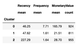
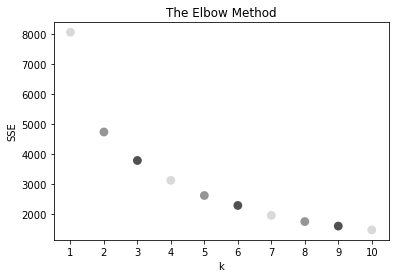
K (the number of clusters) in the K-means - hyperparameter. In our example based on elbow method we selected 3 clusters: 0 - loyal, 1 - new, 2 - churned.
Elbow method - common way to choose K optimally: we plot the sum of squared errors (SSE) for various K values and choose the K value at which the SSE decline slopes change significantly between before and after the value. In the retail example below the K value 3 stands for 3 clusters, because after the third cluster is the function in elbow method already linear.
1. Get the data
# Import The Libraries import pandas as pd import matplotlib.pyplot as plt import numpy as np !pip install xlrd !pip install openpyxl # Import The Dataset, Use dataset: https://archive.ics.uci.edu/ml/datasets/online+retail
df = pd.read_excel("retail_example.xlsx", engine="openpyxl") df = df[df['CustomerID'].notna()] df.head()
2. Sample data
# Sample the dataset
df_fix = df.sample(10000, random_state = 42)
# Convert to show date only
from datetime import datetime
df_fix["InvoiceDate"] = df_fix["InvoiceDate"].dt.date
# Create TotalSum colummn
df_fix["TotalSum"] = df_fix["Quantity"] * df_fix["UnitPrice”]
# Create date variable that records recency
import datetime
snapshot_date = max(df_fix.InvoiceDate) + datetime.timedelta(days=1)
# Aggregate data by each customer
customers = df_fix.groupby(['CustomerID']).agg({
'InvoiceDate': lambda x: (snapshot_date - x.max()).days,
'InvoiceNo': 'count',
'TotalSum': 'sum’})
# Rename columns
customers.rename(columns = {'InvoiceDate': 'Recency',
'InvoiceNo': 'Frequency',
'TotalSum': 'MonetaryValue'}, inplace=True)

from scipy import stats
customers_fix = pd.DataFrame()
customers_fix["Recency"] = stats.boxcox(customers['Recency'])[0]
customers_fix["Frequency"] = stats.boxcox(customers['Frequency'])[0]
customers_fix["MonetaryValue"] = pd.Series(np.cbrt(customers['MonetaryValue'])).values
customers_fix.tail()
3. Normalize data
# Import library to normalize the data
from sklearn.preprocessing import StandardScaler
# Initialize the Object
scaler = StandardScaler()
# Fit and Transform The Data
scaler.fit(customers_fix)
customers_normalized = scaler.transform(customers_fix)
# Assert that it has mean 0 and variance 1
print(customers_normalized.mean(axis = 0).round(2)) # [0. -0. 0.]
print(customers_normalized.std(axis = 0).round(2)) # [1. 1. 1.]
4. Fit model
!pip install seaborn
import seaborn as sns
# Elbow Method , the first 3 clusters are the most significant, other are more linear
from sklearn.cluster import KMeans
sse = {}
for k in range(1, 11):
kmeans = KMeans(n_clusters=k, random_state=42)
kmeans.fit(customers_normalized)
sse[k] = kmeans.inertia_ # SSE to closest cluster centroid
plt.title('The Elbow Method')
plt.xlabel('k')
plt.ylabel('SSE')
sns.pointplot(x=list(sse.keys()), y=list(sse.values()))
plt.show()

# fit the model
model = KMeans(n_clusters=3, random_state=42) model.fit(customers_normalized) model.labels_.shape 5. Create clusters
# Set colors to legend of 3 clusters sns.color_palette("Greys", 3) palette=sns.color_palette("Greys", 3)

customers["Cluster"] = model.labels_ customers.groupby('Cluster').agg({ 'Recency':'mean', 'Frequency':'mean', 'MonetaryValue':['mean', 'count']}).round(2) # Create the dataframe df_normalized = pd.DataFrame(customers_normalized, columns=['Recency', 'Frequency', 'MonetaryValue']) df_normalized['ID'] = customers.index df_normalized['Cluster'] = model.labels_ # Melt The Data df_nor_melt = pd.melt(df_normalized.reset_index(), id_vars=['ID', 'Cluster'], value_vars=['Recency','Frequency','MonetaryValue'], var_name='Attribute', value_name='Value') df_nor_melt.head() 6. Data insight and visualisation
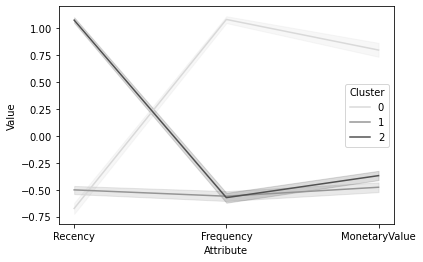
# Visualise clusters sns.lineplot('Attribute', 'Value', hue='Cluster', data=df_nor_melt , palette=palette )

cluster 0 - loyal customer - frequent, spend more, and they buy the product recently.
cluster 1 - new customer - is less frequent, less to spend, but they buy the product recently.
cluster 2 - churned customer - is less frequent, less to spend, and they buy the product at the old time.
Comments