The purpose of this contribution is to create random geometric graph (RDG). We generate the random edge values for lollipop graph and calculate the centrality.
1. Theory
Random geometric graphs (RGG) are the basic spatial networks constructed by randomly placing N nodes in some metric space (according to a specified probability distribution, e.g. Lollipop) and connecting each two nodes (vertices, points) by a link (edge, line).
Centrality is a number or ranking assigned to each node within a graph based on the node position. Centrality is an average length of the shortest path between the node and all other nodes in the graph. More central node has higher centrality value (higher vertex value) and is closer to all other nodes.
Lollipop graph is an example of geodetic graphs (other geodetic graphs include barbell graphs, cacti graphs, odd cycle graphs, trees, triangular snake graphs, windmill graphs, … ). Lollipop graphs can be used the same as bar chart, they are their advanced version. Each bar is replaced with a line and a dot at the end. Lollipop and bar charts can compare items, categories, present rank, show time trend. The lollipop graph consists of 2 components a complete graph called clique and a path graph. L (m ,n) is a lollipop graph with an m-node complete graph and n-node path graph. All lollipop graphs are determined by their Q-spectra.
It is interesting to focus on modularity as well. Modularity is a measure of density in network, modularity number is the strength of division of a network into modules (groups, clusters, communities). Low modularity number indicates the dense connections in cluster (nodes are near, k distance parameter is small), high modularity numbers mean far connections between nodes in community (k distance parameter is higher).
2. Python code
2.1. Install and import the needed libraries.
%matplotlib inline
from random import sample
import networkx as nx
import matplotlib.pyplot as plt
2.2. Generate radom edge list
It is possible to generate the random edge list to draw the lollipop graph. The syntax is networkx.lollipop_graph(m,n), where m is a number of nodes in graph clique and n is a number of nodes in path graph.
G = nx.lollipop_graph(100, 10)
for line in nx.generate_edgelist(G, data=False):
... print(line)
Streaming output truncated to the last 5000 lines.
0 21
0 22
0 23
0 24
0 25
0 26
2.3. Clean the data
In many cases you need to remove randomly selected nodes to make example fast. For lollipop graph you must keep them to see the initial path, not only the clique.
# num_to_remove = int(len(G) / 1.5)
# nodes = sample(list(G.nodes), num_to_remove)
# G.remove_nodes_from(nodes)
For lollipop graph you do not remove low-degree nodes, but you keep them to see the path in the graph.
# low_degree = [n for n, d in G.degree() if d < 10]
2.4. Connected components
Create the list of connected components and see the largest connected component. The list of largest connected components is used to calculate the centrality and the community index.
components = nx.connected_components(G)
list(nx.connected_components(G))
[{3,
4,
5,
16,....
components
<generator object connected_components at 0x7fbbfcfc0750>
# largest connected component
largest_component = max(components, key=len)
H = G.subgraph(largest_component)
2.5. Compute the centrality
Nodes that more frequently lie on shortest paths between other nodes will have higher betweenness centrality scores, nodes 98 or 99 are more impactful (bigger size in graph, higher vertex weight) than nodes 1 or 2 (smaller size in graph, smaller vertex weight). In the code we use the centrality value to size each node in the graph.
centrality = nx.betweenness_centrality(H, k=10, endpoints=True)
centrality
{0: 0.009174311926605505,
1: 0.009174311926605505,
2: 0.009174311926605505,
...
97: 0.009174311926605505,
98: 0.10825688073394496,
99: 0.18256880733944955,
100: 0.17522935779816515,
...
2.6. Compute the community structure
Use the new labels to classify colors for graph. Nodes with similar community index have similar colors. For classification is used Label propagation methodology, which is a semi-supervised machine learning algorithm that assigns vertex labels to previously unlabeled data points.
lpc = nx.community.label_propagation_communities(H)
community_index = {n: i for i, com in enumerate(lpc) for n in com}
i=len(community_index)
# Color mapping
import seaborn as sns
from matplotlib.colors import ListedColormap
# color_palette = sns.cubehelix_palette(i)
color_palette = sns.color_palette("Greys",(i))
2.7. Create Lollipop graph
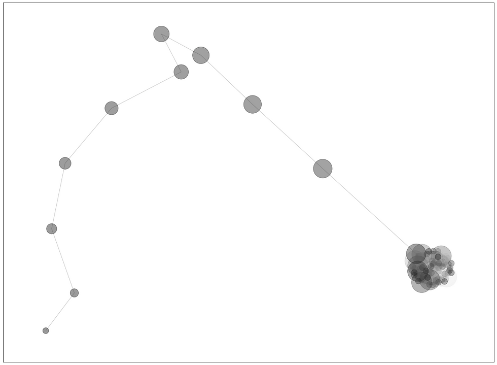
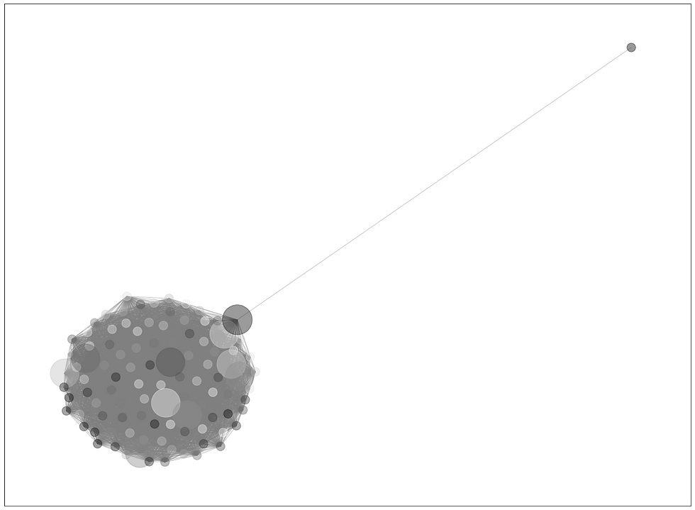
You can select the required layout, sizes and colors. Parmeter k stands for modularity. To increase the distance between nodes in clique, increase the modularity size, e.g. from k=0.15 to k=2.1.
fig, ax = plt.subplots(figsize=(20, 15))
pos = nx.spring_layout(H, k=0.15, seed=4572321)
node_color = [community_index[n] for n in H]
node_size = [v * 20000 for v in centrality.values()]
nx.draw_networkx(
H,
pos=pos,
with_labels=False,
node_color=color_palette,
node_size=node_size,
edge_color="grey",
alpha=0.4
)
# prepare to save the figure without borders
plt.axis('off')
# set higher pad inches for miniature icon for webpage
plt.savefig('data.jpg', dpi=400, bbox_inches='tight',pad_inches=3.9,frameon=None)
Sample graph below illustrates a distance irregular vertex labelling of the lollipop graph L100,10 with distance irregularity strength 0.15.

Sample graph of (100,1) lollipop graph, k=0.15, looks like this:

3. References
https://networkx.org/documentation/networkx-1.1/_downloads/networkx_reference.pdf
https://en.wikipedia.org/wiki/Lollipop_graph
https://networkx.org/documentation/stable/index.html
https://www.youtube.com/watch?v=PouhDHfssYA
https://github.com/sepinouda/Intro_to_Data_Science/blob/main/Lecture%204/Network%20Analysis/NetworkX.ipynb
https://networkx.org/documentation/stable/auto_examples/geospatial/plot_polygons.html
https://github.com/sepinouda/Intro_to_Data_Science/tree/main/Lecture%204/Network%20Analysis
https://programminghistorian.org/en/lessons/exploring-and-analyzing-network-data-with-python
https://conference.scipy.org/proceedings/SciPy2008/paper_2/full_text.pdf
https://www.sciencedirect.com/science/article/pii/S0021980067801042
https://www.geeksforgeeks.org/lollipop-graph-in-python-using-networkx-module/
https://mathworld.wolfram.com/DodecahedralGraph.html
https://www.brainkart.com/article/One-Dimensional-Finite-Element-Analysis--Beam-Element_5949/
https://xlinux.nist.gov/dads/HTML/selfloop.html
https://en.wikipedia.org/wiki/Eigenvalues_and_eigenvectors
https://networkx.org/documentation/stable/reference/algorithms/generated/networkx.algorithms.community.modularity_max.greedy_modularity_communities.html
https://thegraph.com/docs/en/developing/creating-a-subgraph/
https://subgraph.com
https://xlinux.nist.gov/dads/HTML/subgraph.html
https://www.researchgate.net/publication/267037782_Circular_Tree_Drawing_by_Simulating_Network_Synchronisation_Dynamics_and_Scaling
https://en.wikipedia.org/wiki/Centrality
https://en.wikipedia.org/wiki/Katz_centrality
https://en.wikipedia.org/wiki/Random_geometric_graph
https://data.doi.gov/organization/lcc-network
https://www.sciencedirect.com/science/article/pii/S0012365X08005931
https://pegasus.uprm.edu/xryong/RecentPublications/ZhLiZhYoDM09.pdf
https://neo4j.com/docs/graph-data-science/current/algorithms/betweenness-centrality/
https://www.programcreek.com/python/example/89598/networkx.betweenness_centrality
https://www.researchgate.net/publication/4866317_Which_Graphs_are_Determined_by_their_Spectrum/link/5e578d3492851cefa1c7fe46/download
https://en.wikipedia.org/wiki/Label_propagation_algorithm
Comentarios